Part 6 Probability Distributions, Unbalanced datasets, and averaging
- Rodrigo Ledesma
- May 15, 2022
- 13 min read
Updated: May 19, 2022
Random Oversampling, SMOT, Random Undersampling, Near Miss
Welcome back one more time to my series of posts. On our last adventure, we began facing problems related to the metrics obtained after training our model. We learned last time how to evaluate or logistic regression model using performance metrics such as accuracy, recall, precision, F1, and ROC.
If you are new to my blog welcome, let me tell you very briefly that the objective of these articles is to use Machine Learning to predict how much time an average customer will take waiting in line to ride a roller coaster at Disney World or Universal Studios. This with the purpose of optimizing their experience.

In Part 5 we trained a Logistic Regression Model and used it to make some predictions. Based on those predictions we used different performance metrics to test how good our model is. The results we obtained were bad. And now we will be explaining why. But before we get too technical, let’s introduce a simple topic. Symmetric and skewed data

When plotting the distribution of a dataset, we can find ourselves with the three cases shown above. The first case that looks like a bell is an example of symmetric data, mean mode and median are in the middle. Of course, this is an extraordinary case, it is extremely difficult that a normal dataset has this distribution without any type of manipulation. Then we have negative and positive skewed data, which are the other two representations, where most of our data will be leaning towards one side of the graph and also the mean, mode, and median.
With this in mind let’s take a look at the distribution of our waiting times for the harry potter ride:
import pandas as pdhp_ohe = pd.read_csv("harryPotterCleanOHE.csv")
hp_oe = pd.read_csv("harryPotterCleanOE.csv")
hp_me = pd.read_csv("harryPotterClean.csv")time_counts = pd.DataFrame(hp_me['Harry_Potter_and_the_Forbidden'].value_counts())
time_countsdata = {'time':[  0, 5, 10, 11, 15, 20, 25, 30, 35, 40, 45, 50, 55, 60, 65, 70, 75, 80, 85, 90, 95, 100, 105, 110, 115, 120, 125, 130, 135, 145, 150, 180,],
        'count':[1, 66, 2922, 1, 2078, 1258, 1447, 249, 1323, 437, 1391, 399, 301, 1148, 222, 115, 886, 113, 115, 614, 75, 144, 138, 76, 28, 196, 2, 1, 3, 1, 10, 5,]}
df=pd.DataFrame(data)
What we did with this code is very simple, read the csv file and create a dataframe that contains all the different times ( 5 min, 10 min…) and how many times each category repeats:
print(sorted(Counter(y).items()))[(0.0, 1), (5.0, 66), (10.0, 2922), (11.0, 1), (15.0, 2078), (20.0, 1258), (25.0, 1443), (30.0, 249), (35.0, 1319), (40.0, 437), (45.0, 1385), (50.0, 397), (55.0, 301), (60.0, 1145), (65.0, 222), (70.0, 115), (75.0, 886), (80.0, 113), (85.0, 115), (90.0, 613), (95.0, 75), (100.0, 144), (105.0, 138), (110.0, 76), (115.0, 28), (120.0, 196), (125.0, 2), (130.0, 1), (135.0, 3), (145.0, 1), (150.0, 10), (180.0, 5)]And for being more visual, let’s create a histogram:

As you can see we have a right-skewed distribution (positive skew). This means one simple thing. We have too many values on small categories, in other words, most of the time, this ride takes less than 100 minutes, and there are very few observations containing information of times bigger than 2 hours. This is called an unbalanced dataset.
Density Plot
To make our data look more appealing and make a match with the representations of the skews, let’s make a density plot, specifically a kernel density plot. The density plot is a continuous representation of the histogram, and it is created by calculating a Gaussian curve on each and every point on the x-axis. After all the Gaussian curves are calculated, the function will add them up and draw a single curve. If this is difficult to imagine, please take a look at the next image, the Gaussian curves are painted in red, while the density function is painted in blue (this is a generic example and has nothing to do with our data)

So, for each point in the x-axis we are going to calculate its mean and standard deviation, and we will plot the curve (red). When all red curves are calculated, then we will plot the blue line, which is the sum of all individual curves. This blue lines is our density function and it ill help us to calculate the probability of certain events. Let’s do some python magic to plot our density function based on the ride’s data and come back to the beautiful maths behind it.
# Import the libraries
import matplotlib.pyplot as plt
import seaborn as sns# Density Plot and Histogram of all arrival delays
sns.distplot(hp_me['Harry_Potter_and_the_Forbidden'], hist=True,                      kde=True,
             bins=int(180/5), color = 'darkblue',
             hist_kws={'edgecolor':'black'},
             kde_kws={'linewidth': 4})
The code is quite self-explanatory but generally speaking, we are asking the function to plot a histogram of the ride’s time and also the kernel density distribution, with a certain amount of bins and with specific colors for the lines and bins. Easy as winning against the Senators isn’t it? Let’s see the result:

Now it is important to discuss that the y-axis does not represent the probability of an event, it is its density. Let’s make a hypothetical case and say that based on this data, we will be visiting Universal Studios with our crush (who is a Potterhead) and we want to make sure that we get the best time, so let's calculate the probability of this ride has a waiting time equal or smaller to an hour. For this calculation, we need to use the area under the curve and perform the following integral. Saying that the blue line is a function f(x):

The result of that operation will give us the probability of waiting for less than an hour in line, we can impress our crush by calculating this same expression for all the harry potter rides and visiting the one which has the biggest probability.
Balanced vs Unbalanced dataset
A machine learning model can be nudged into a certain direction if we train it with a huge amount of information from one case, and small amounts from another. In this specific example, our initial dataset is unbalanced, which means that each category has a different quantity of values. Most of our data is concentrated in categories smaller than 100 minutes in the waiting time dataset. Once we trained the model, it will make most of its predictions in this range, because most of its training was based on these ranges. It is as if we are practicing karate, and our sensei only teaches us how to kick and superficially mentions how to punch. When we are in a battle, we will feel more comfortable kicking than punching and we will do it most of the time.
A balanced dataset is a set of values whose categories contain approximately the same amount of data. So in this case our goal will be to balance our data and then retrain our model.
We are going to be testing 4 different methods of oversampling (creating more data for the minority classes) and undersampling (deleting data from the majority classes).
Random Oversampling
SMOTE (Synthetic Minority Oversampling Technique)
Random Under-Sampling
Near Miss Under-Sampling
I followed the tutorial of Amy GrabNGoInfo it is excellent, for more examples, look at how she creates the data. It is a complementary point of view of that you will be learning today. She uses a binary classification and I used a multiclass.
Four Oversampling And Under-Sampling Methods For Imbalanced Classification Using Python
Random Oversampling, SMOTE, Random Under-sampling, and NearMiss
medium.com
After citing my references, now we can move on with the code. Just FYI the link to my google colab notebook and my datasets are at the bottom of the article.
So let’s start at the very beginning, let’s import the dataFrames and make the splits as if we were starting from zero.
# Oversampling and under sampling
from sklearn.model_selection import train_test_split
from imblearn.over_sampling import RandomOverSampler, SMOTE
from imblearn.under_sampling import RandomUnderSampler, NearMiss
from collections import Counterdef getXandY(df):
    df.drop(df.tail(20).index,inplace=True)
    x = df.drop(['Harry_Potter_and_the_Forbidden','Unnamed: 0'],axis=1)
    y = df.Harry_Potter_and_the_Forbidden
    return(x,y)def trainTest(x,y):
    X_train, X_test, y_train, y_test = train_test_split(x, y, test_size=0.30, shuffle=True)
    return(X_train, X_test, y_train, y_test)x,y=getXandY(hp_me)
X_train, X_test, y_train, y_test = trainTest(x,y)
Now let’s use the Random Oversampling technique
This function will analyze the number of elements each class has and copy random elements of the smaller classes until each class has the same number of elements as the biggest class. For instance, in this case, our biggest class contains 2064 elements, it belongs to the 10 min class. So our function will analyze this and go class by class, randomly duplicating values until each class contains 2064 elements. We will do this with the following code:
# Randomly over sample the minority class
ros = RandomOverSampler(random_state=42)
X_train_ros, y_train_ros= ros.fit_resample(X_train, y_train)
# Check the number of records after over sampling
print(sorted(Counter(y_train_ros).items()))[(0.0, 2064), (5.0, 2064), (10.0, 2064), (11.0, 2064), (15.0, 2064), (20.0, 2064), (25.0, 2064), (30.0, 2064), (35.0, 2064), (40.0, 2064), (45.0, 2064), (50.0, 2064), (55.0, 2064), (60.0, 2064), (65.0, 2064), (70.0, 2064), (75.0, 2064), (80.0, 2064), (85.0, 2064), (90.0, 2064), (95.0, 2064), (100.0, 2064), (105.0, 2064), (110.0, 2064), (115.0, 2064), (120.0, 2064), (130.0, 2064), (135.0, 2064), (145.0, 2064), (150.0, 2064), (180.0, 2064)]
Perfect! Now each class contains exactly 2064 elements. Our dataset is balanced. Something very important to highlight (and something I got wrong in my ML class) is that we will only be oversampling the TRAIN dataset. please don’t touch the test or validation dataset.
Now there is something worth analyzing.
Do you think it is really necessary to use extremely big values? Specifically those bigger than 2 hours? They are less than 30 elements, they are known as outliers. Outliers in this case represent a minuscule part of our dataset and will cause some troubles when training the model. Also, 0 minutes does not have a lot of sense, so let’s have 2 different datasets, one with outliers and one without, and at the end of the day let’s compare the performance of the model trained with both datasets.
Complete case:
Now let's retrain our model with the randomly oversampled data, including outliers, and compare the result to our base
from sklearn.linear_model import LogisticRegression
from sklearn import metricslogisticRegr = LogisticRegression(max_iter=20000)
logisticRegr.fit(X_train_ros, y_train_ros).decision_function(X_test)
y_pred=logisticRegr.predict(X_test)from sklearn.metrics import classification_report
print(classification_report(y_test, y_pred))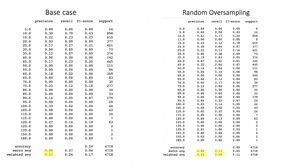
Let’s see what the classification report states, its a complete performance metric report in a single line of code, it gives the precision, recall, and F1 score of each class, also it averages in macro and weighted (macro assigns the same weight to all the classes, we will see it shortly) together with accuracy. Our left table is the base, the original dataset without oversampling. On the right, we can see the oversampled analysis with random oversampling. As you can appreciate there is not a lot of improvement, actually there the F1 score is worse. So this means we should modify our data or use a different oversampling method. Before we try a different method let's do a little trick. I am going to delete the values of zero and also delete values bigger than 120 mins, re-run the oversampling, and analyze the metrics.
Trimmed dataset
This will be easy and quick let's delete all rows which contain outliers like 0 mins or 180.
hp_clean = hp_me[hp_me.Harry_Potter_and_the_Forbidden != 0] #delete rows with 0 min
hp_clean = hp_clean[hp_clean.Harry_Potter_and_the_Forbidden != 180]
hp_clean = hp_clean[hp_clean.Harry_Potter_and_the_Forbidden != 150]
hp_clean = hp_clean[hp_clean.Harry_Potter_and_the_Forbidden != 145]
hp_clean = hp_clean[hp_clean.Harry_Potter_and_the_Forbidden != 135]
hp_clean = hp_clean[hp_clean.Harry_Potter_and_the_Forbidden != 130]
hp_fin_clean = hp_clean[hp_clean.Harry_Potter_and_the_Forbidden != 125]print(sorted(hp_fin_clean.Harry_Potter_and_the_Forbidden.unique()))[5.0, 10.0, 11.0, 15.0, 20.0, 25.0, 30.0, 35.0, 40.0, 45.0, 50.0, 55.0, 60.0, 65.0, 70.0, 75.0, 80.0, 85.0, 90.0, 95.0, 100.0, 105.0, 110.0, 115.0, 120.0]
Once trimmed the original dataset, let's divide it into X and Y and retrain the Logistic Regression model
xTrim,yTrim=getXandY(hp_fin_clean)
X_trainTrim, X_testTrim, y_trainTrim, y_testTrim = trainTest(xTrim,yTrim)# Randomly over sample the minority class
ros = RandomOverSampler(random_state=42)
X_train_rosTrim, y_train_rosTrim= ros.fit_resample(X_trainTrim, y_trainTrim)
# Check the number of records after over sampling
print(sorted(Counter(y_train_rosTrim).items()))
Once it is trained, let's see the performance metrics and compare them with our last experiment and the base case.
logisticRegr.fit(X_train_rosTrim, y_train_rosTrim).decision_function(X_testTrim)
y_predTrim=logisticRegr.predict(X_testTrim)
print(classification_report(y_testTrim, y_predTrim))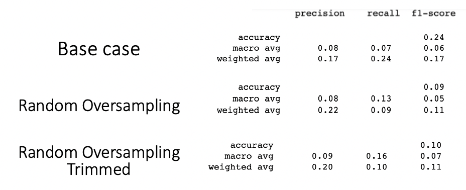
Synthetic Minority Oversampling Technique SMOTE
It seems like only copy and pasting random values inside the imbalanced classes does not really worked. But why? Well, the random oversampling grabs the class subset and chooses randomly some values and duplicates them, but what happens if we only have 10 values on a class? Well the information will be the same, there will not be any added information while training the model. For example if we show a picture of the same Chihuahua dog to an alien it will understand that’s a dog, but it will only recognize it, when we give him a picture of a huskey the alien will not understand what it is.
For solving that problem, SMOT technique was introduced in 2002. This technique consists on making an spacial analysis of the data, you can imagine a 2D plane containing the values of the class. In this space the SMOT technique will apply a kind of clustering algorithm like this:
Smot will choose a random sample in the minority class
It will then look for its neighbors
Once it finds the neighbors it will create an imaginary line between the chosen value and the neighbor, and in this line, it will create a new data point.
If this sounds familiar it is because SMOT is using k nearest neighbors algorithm which we will discuss later on in this blog.
With this in mind please feel free to read this great article that contains a detailed explanation of how it works:
https://machinelearningmastery.com/smote-oversampling-for-imbalanced-classification/
From this article I obtained these images.

Now it is clear how the process works, so let’s use our waiting times data to try it out. The SMOTE technique requires us to have a minimum amount of values inside each class, so I will delete those classes that contain 5 or less data points first.
x,y=getXandY(hp_me)
X_train, X_test, y_train, y_test = trainTest(x,y)
print(sorted(Counter(y_train).items()))[(0.0, 1), (5.0, 47), (10.0, 2008), (11.0, 1), (15.0, 1468), (20.0, 875), (25.0, 1024), (30.0, 178), (35.0, 898), (40.0, 297), (45.0, 976), (50.0, 259), (55.0, 207), (60.0, 802), (65.0, 156), (70.0, 84), (75.0, 611), (80.0, 78), (85.0, 76), (90.0, 444), (95.0, 48), (100.0, 103), (105.0, 107), (110.0, 51), (115.0, 23), (120.0, 141), (125.0, 2), (130.0, 1), (135.0, 1), (150.0, 7), (180.0, 5)]# Let's clean our data, as the smote technique requires the class to have at least n neighbors
hp_clean = hp_me[hp_me.Harry_Potter_and_the_Forbidden != 0]
hp_clean = hp_clean[hp_me.Harry_Potter_and_the_Forbidden != 11]
hp_clean = hp_clean[hp_clean.Harry_Potter_and_the_Forbidden != 180]
hp_clean = hp_clean[hp_clean.Harry_Potter_and_the_Forbidden != 145]
hp_clean = hp_clean[hp_clean.Harry_Potter_and_the_Forbidden != 135]
hp_clean = hp_clean[hp_clean.Harry_Potter_and_the_Forbidden != 130]
hp_fin_clean = hp_clean[hp_clean.Harry_Potter_and_the_Forbidden != 125]x_Smote,y_Smote=getXandY(hp_fin_clean)
X_train, X_test, y_train, y_test = trainTest(x_Smote,y_Smote)
# Randomly over sample the minority class
smote = SMOTE(random_state=42)
X_train_Smote, y_train_Smote= smote.fit_resample(X_train, y_train)
# Check the number of records after over sampling
print(sorted(Counter(y_train_Smote).items()))[(5.0, 2050), (10.0, 2050), (15.0, 2050), (20.0, 2050), (25.0, 2050), (30.0, 2050), (35.0, 2050), (40.0, 2050), (45.0, 2050), (50.0, 2050), (55.0, 2050), (60.0, 2050), (65.0, 2050), (70.0, 2050), (75.0, 2050), (80.0, 2050), (85.0, 2050), (90.0, 2050), (95.0, 2050), (100.0, 2050), (105.0, 2050), (110.0, 2050), (115.0, 2050), (120.0, 2050), (150.0, 2050)]
Now we are ready, let’s train out Logistic Regression model one more time using a base case and also using the Smote oversampled data and let’s compare the performance.
Train and evaluate our model
logisticRegr.fit(X_train_Smote, y_train_Smote).decision_function(X_test)
y_pred_Smote=logisticRegr.predict(X_test)
print(classification_report(y_test, y_pred_Smote))
Left table contains the base results and right table contains the metrics using SMOTE oversampling
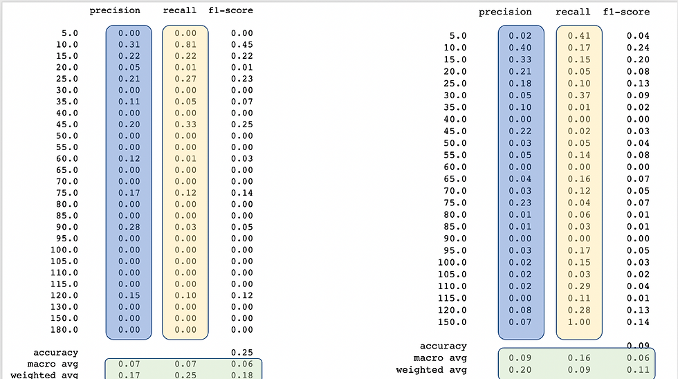
Ok, let’s analyze. Results are not overwhelming, but maybe this little push will be the one that gets you to win a kaggle competition one day. First improvement is while analyzing the precision, most of the classes improved their precision and also the amount of classes with zero precision were drastically reduced. Recall is a different thing, the amount of classes with recall cero was reduced but also the recall of some classes was also reduced, let’s remember our data is better distributed now. We can appreciate an important increase in the average analysis (those in green) for precision and recall.
Undersampling methods
Ok now we have seen how oversampling improves our analysis, let’s see what happens when we instead of creating new values, delete values to even the amount of data.
The first technique we will see is random undersampling
We have already trimmed our dataset so let’s see how the undersampling technique treats our data.
# Randomly under sample the majority class
rus = RandomUnderSampler(random_state=42)
X_train_rus, y_train_rus= rus.fit_resample(X_train, y_train)
# Check the number of records after under sampling
print(sorted(Counter(y_train_rus).items()))[(5.0, 7), (10.0, 7), (15.0, 7), (20.0, 7), (25.0, 7), (30.0, 7), (35.0, 7), (40.0, 7), (45.0, 7), (50.0, 7), (55.0, 7), (60.0, 7), (65.0, 7), (70.0, 7), (75.0, 7), (80.0, 7), (85.0, 7), (90.0, 7), (95.0, 7), (100.0, 7), (105.0, 7), (110.0, 7), (115.0, 7), (120.0, 7), (150.0, 7)]
LOL! There was a class with 7 datapoints, this is not going to work so let’s first treat our trimmed dataset. But let’s not get rid of more information by deleting rows, lets better join those who have similar waiting times, such as 5, 10 and 15 min will be considered 10 mins, and so on.
Ok let me just give you the code I used to manipulate the data, might not be the most efficient, but I like it.
#replace values with nearest decimal a=hp_fin_clean.Harry_Potter_and_the_Forbidden.replace([5, 15, 25, 35, 45, 55, 65, 75, 85, 95, 105, 115, 120, 110, 150], [10,10, 20, 30, 40, 50, 60, 70, 80, 90, 100, 100, 100, 100, 100])
#create a df and drop the last column
df=pd.DataFrame(a)
hp2=hp_fin_clean.drop('Harry_Potter_and_the_Forbidden',axis=1)
#concatenate the new and replaced df and clean
hp3=pd.concat([hp2, df], axis=1)
hp4=hp3.drop('Unnamed: 0',axis=1)
Before we try undersampling, let’s see how our values are going:
x_und,y_und=getXandY2(hp4)
X_train_und, X_test_und, y_train_und, y_test_und = trainTest(x_und,y_und)
print(sorted(Counter(y_train_und).items()))[(10.0, 3555), (20.0, 1878), (30.0, 1075), (40.0, 1257), (50.0, 482), (60.0, 944), (70.0, 698), (80.0, 166), (90.0, 459), (100.0, 399)]
Not the best idea yet, the smallest value is 166 followed by 399, so let’s look for a way to make the smallest class a little bigger. I will be merging 70, 80 and 90 into 100, and 50 into 60.
b=hp4.Harry_Potter_and_the_Forbidden.replace([80, 90, 50,70],
                                             [100, 100, 60,100])
df2=pd.DataFrame(b)
hp5=hp4.drop('Harry_Potter_and_the_Forbidden',axis=1)
hp6=pd.concat([hp5, df2], axis=1)
x_und2,y_und2=getXandY2(hp6)
X_train_und2, X_test_und2, y_train_und2, y_test_und2 = trainTest(x_und2,y_und2)
# Randomly under sample the majority class
rus = RandomUnderSampler(random_state=42)
X_train_rus2, y_train_rus2 = rus.fit_resample(X_train_und2, y_train_und2)
# Check the number of records after under sampling
print(sorted(Counter(y_train_rus2).items()))[(10.0, 1077), (20.0, 1077), (30.0, 1077), (40.0, 1077), (60.0, 1077), (100.0, 1077)]
Now it looks more reasonable, let’s try it out :
logisticRegr.fit(X_train_rus2, y_train_rus2).decision_function(X_test_und2)
y_pred_rus2=logisticRegr.predict(X_test_und2)
print(classification_report(y_test_und2, y_pred_rus2))
Random undersampling with 6 classes
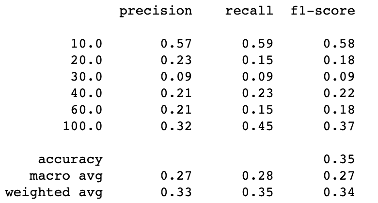
This is way better! everything has improved. Just for fun let’s see what happened before doing this last trick.
logisticRegr.fit(X_train_rus, y_train_rus).decision_function(X_test_und)
y_pred_rus=logisticRegr.predict(X_test_und)
print(classification_report(y_test_und, y_pred_rus))
Random undersampling with 10 classes
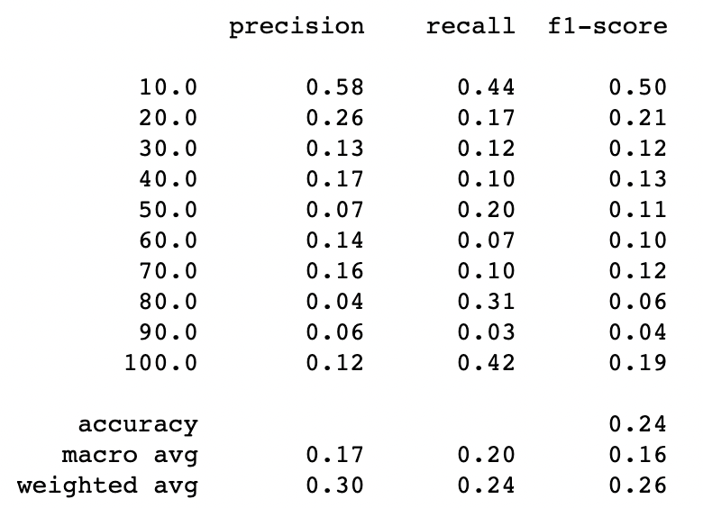
There is an overall improvement when reducing the number of classes from 10 to 6, this is so far the best performance we have had so far. So now we will be trying a new undersampling technique and at the end, we will re run the oversampling techniques, now using the dataset with less classes.
Under-Sampling Using NearMiss
This technique uses K Nearest Neighbors to undersample the dataset. There are 3 versions of the algorithm and we will be testing them all. But before let’s give a short description of each variation.
“NearMiss-1 selects the positive samples for which the average distance to the N closest samples of the negative class is the smallest.”
“NearMiss-2 selects the positive samples for which the average distance to the N farthest samples of the negative class is the smallest.”
“NearMiss-3 is a 2-steps algorithm. First, for each negative sample, their M nearest neighbors will be kept. Then, the positive samples selected are the one for which the average distance to the N nearest-neighbors is the largest.”
I have been a little lazy and I have repeated the code a lot, so let’s define some beautiful functions for undersampling and creating the model:
from imblearn.under_sampling import NearMiss#This function will use the nearmiss technique to undebalance the training data, create a logReg model and print its metrics
def nM(version, x_train, y_train, X_test, y_test):
    #undersample training datasets
    X_train_nearmiss, y_train_nearmiss= version.fit_resample(x_train, y_train)
    # Check the number of records after over sampling
    print(sorted(Counter(y_train_nearmiss).items()))

    #fit logreg
    logisticRegr.fit(X_train_nearmiss, y_train_nearmiss).decision_function(X_test)
    y_pred_nM=logisticRegr.predict(X_test)
    print(classification_report(y_test, y_pred_nM))
This is an example of how I am running the functions:
# Under sample the majority class
nearmiss1 = NearMiss(version=1)
nM(nearmiss1, X_train_und2, y_train_und2, X_test_und2, y_test_und2)
Easy! Like winning a match against the Ottawa Senators! Now let’s take a look at the results:

The nearMiss version 2 does not perform the best, so we will be using version 1 as it has a slightly better result for this dataset than version 3.
Before we finish, let’s repeat the Oversampling techniques with the reduced dataset of only 6 classes:
ros = RandomOverSampler(random_state=42)
smote = SMOTE(random_state=42)def overSampling(X_train, y_train, X_test, y_test, method):
    X_train_os, y_train_os= method.fit_resample(X_train, y_train)
    # Check the number of records after over sampling
    print(sorted(Counter(y_train_os).items()))logisticRegr.fit(X_train_os, y_train_os).decision_function(X_test)
    y_pred=logisticRegr.predict(X_test)
    print(classification_report(y_test, y_pred))
Random Oversampling with 6 classes

SMOT with 6 classes
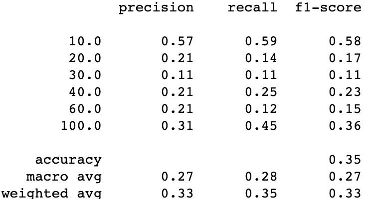
And one more time we can see that SMOT is better than random oversampling, but we still need to compare if oversampling is better than undersampling. Let’s compare the SMOT technique with the NearMiss Ver 1 using only 6 classes.

Results are extremely similar but SMOT is slightly better in recall with weighted average and also in the accuracy. So we might say we have a winner.


Comments