Part 8 Feature Selection Discrimination
- Rodrigo Ledesma
- May 15, 2022
- 7 min read
Updated: May 24, 2022
Hello and welcome back! In the last post we analyzed and learned how to implement a Principal Component Analysis using Sklearn and our waiting times' data, in this post we will do a similar analysis but now we will be discriminating which of the feature selection techniques obtained in Part 4
(https://medium.com/@rledesma.itesm/a-magical-day-in-disney-with-machine-learning-part-4-feature-selection-techniques-374be81b0bae) will be the best approach for our data.

If this is the first time you visit my blog, the purpose of this series of articles is intended to create a Machine Learning model to predict how long will it take an average visitor to wait in line at a Disney or Universal park before they can ride their favorite rollercoaster and with this information, optimize their visit by scheduling parks in the day where their favorite parks are less crowded.
If you remember in Part 4 we used 4different techniques to discriminate which variables were the most relevant for our dataset (Correlation, Mutual Information, Variance Threshold, and MRMR) we also tested different variations of some methods such as the Pearson and Kendall's correlation. What we will do in this article, is gradually analyze the performance of our model with different combinations of variables in the order that the methods suggested.
Before we begin, I will just explain one thing. This is a little bit of philosophy and physics.
Einstein’s phase
It is widely known that it is said that Einstein once said “God does not play dice with the universe”. If it is true or not is out of the scope of this article. But I agree with him. In my opinion, the only reason why we use probability and statistics is that we don’t have tools that are precise or powerful enough to determine the final state of a system given a number of variables. So given our limited understanding and technology, the only resource we can use is statistics. Repeat something a lot of times and try to generate a pattern.
In order to have a statistically significant result, I will be repeating 100 times the experiment, storing the results, and making an average out of them to analyze the performance of the model given the set and order of the variables given.
Comparing the results of the encoding methods
Just as a quick reminder we used in Part 4 three different encoding methods (Manual Encoding, One Hot Encoding, and Ordinal Encoding). Each one gave as an output a sorted list where the first features were the most relevant ones for the analysis. Apart from those encoding methods, we used seven feature selection techniques (Pearson correlation, Kendall’s correlation, MRMR, Mutual information for regression, classification and second code, and last Variance Threshold). So my plan is simple, I will be creating a function that will analyze each of the 3 different dataframes (each containing a different encoding methodology). With each encoding method, I will also be analyzing each feature selection technique. Let’s say that for example, I will begin by analyzing Manual Encoding with Pearson correlation.
Step 1: Prepare my data
Step 2: Define the order of the variables based on the result of the analysis
Step 3: Use only the first variable to train the model
Step 4: Analyze the performance metrics and store them in a list
Step 5: Repeat 100 times step 3 and 4, averaging the results on the list
Step 6: Print the average result of the 100 runs
Step 7: Train the model with the two main variables
Step 8: Repeat steps 3 and 4, 100 times and print the average result
Step 9: increase the number of features analyzed in the loop until we use all of the
Step 10: Compare the performance metrics of all the runs and decide which number of variables is the best for that encoding technique
Step 11: Repeat steps 1 to 10 for the other two encoding techniques.
At the end of this exercise, we should have the best encoding method and also the optimal amount of variables to training our model.
Analyzing Manual Encoding
As we said the first step will be, to reorder the position of the features within the dataframe based on the result of the feature selection algorithm. Just to refresh your memory, this was the result of the algorithms for the manual encoding method.

This table can be interpreted as:
With the manual encoding method, after applying the Pearson correlation methodology, the most important variable for the analysis is temperature, the following ones are less important as the table grows. So we will be rearranging our dataframe with respect to these results:
#Variable order in manual correlation:pear_corr = ['temperature', 'holiday', 'day', 'month', 'pressure', 'day.1','report','minute','year','humidity','hour', 'Pandemic']
kend_corr = ['temperature', 'holiday', 'month', 'day', 'pressure', 'day.1', 'report','year', 'minute','humidity','hour','Pandemic']
mutInf_class = ['month','day', 'year', 'hour', 'minute', 'holiday', 'day.1','Pandemic','temperature','humidity','pressure','report']
mutInf_reg = ['month','day','year','hour', 'minute', 'holiday', 'day.1','Pandemic', 'temperature','humidity','pressure','report']
mutInf_class2 = ['day','temperature','month', 'humidity', 'hour', 'day.1','pressure','holiday','year','report','minute','Pandemic']
varThre = ['month','day','year','hour','minute','holiday','day.1',
           'temperature','humidity','pressure','report']
mrmr = ['temperature','day.1','hour','holiday','humidity','day',
        'year','month','pressure','minute','report']method ['Pearson_correlation', 'Kendalls_correlation', 'mutualInformation_classification', 'mutualInformation_reggression', 'mutualInformation_classification2','variableThreshold','MRMR']
Now there comes the most interesting part, add one variable per iteration and repeat the model training and testing 100 times.
smote = SMOTE(random_state=42)def testModel(df,var_order,n_vars):
    for j in tqdm(range(1,n_vars)):
        #split our dataframe into X and Y
        x,y=getXandY(df)
        #create the lists to store metrics
        acc = []
        rec = []
        preci = []
        f1 = []
        for i in range(100):
            #split the dataFrame into test and train
            X_train, X_test, y_train, y_test = trainTest(x,y)
            #Oversample the train dataset with SMOTE
            X_train_os, y_train_os=overSampling(X_train, y_train, y_test, smote)
            #define the variables order
            X_train_os_r = X_train_os[var_order]
            X_test_r = X_test[var_order]
            df1= X_train_os_r.iloc[:, 0:j] #use only part of the variables
            lg = LogisticRegression(max_iter=20000)
            lg.fit(df1, y_train_os).decision_function(X_test_r.iloc[:, 0:j])
            y_pred=lg.predict(X_test_r.iloc[:, 0:j])
            ac=metrics.accuracy_score(y_test, y_pred)
            acc.append(ac)
            p=metrics.precision_score(y_test, y_pred,average='macro')
            preci.append(p)
            r=metrics.recall_score(y_test, y_pred,average='macro')
            rec.append(r)
            f=metrics.f1_score(y_test, y_pred, average='macro')
            f1.append(f)
        print(df1.columns)
        print("For {} features: \n Accuracy: {} \n Precision: {} \n Recall: {} \n F1 score: {}".format(
        j,mean(acc),mean(preci),mean(rec),mean(f1)))
        print(classification_report(y_test, y_pred))
The code looks complicated but it is actually extremely simple and straightforward.
First, we define a function that will receive a dataframe and the order of the variables it should analyze. Inside this function, there will be two different loops. The first one will run 12 times, in each loop one variable will be added to the analysis. In the first loop, we will train the model with only the first feature, in the second loop, we will add the second one, training the model with features [1,2]. In the third loop, we will add the third feature, training the model with vars [1,2,3]. And so on. But now for making sure our results are statistically significant, we will start a second for loop, this one will run 100 times. In this second loop, we will be training and testing the model. Also, we will be saving the performance metrics in an array.
At the end of the second loop (the one that runs 100 times), we will do the averaging of the 100 loops and print the information obtained. This process of repeating and averaging will be repeated for every variable added (in this case 12 times).
order=[pear_corr,kend_corr,mutInf_class, mutInf_reg, mutInf_class2, varThre,mrmr]for i in range(len(order)):
    print('------------------------- Analyzing method {} -------------------------'.format(method[i]))
    print('The variable order is: \n {}'.format(order[i]))
    testModel(hp,order[i],12)
    print('\n \n')
You can find at the end of this post the google colab notebook to try it yourself, also if you visit my GitHub you will be able to find the datasets I used. but please take into consideration that this process is very time-consuming I used a laptop with a GPU and some of the runs took an hour. Especially when I run the one hot encoding where each loop will be repeated 28 times.
If you visit my GitHub you will also find some .txt files where I put the results of the process, as if they were logs. Here I will be just showing some examples and doing an analysis. So let’s see what the program outputs:

So, the output is telling us, that we are analyzing the Pearson correlation for the manual encoding. The order of this specific method is the one in brackets. In this first iteration (1/11) we are only using the variable temperature for training our model, only 1 feature. After the training is done, the average accuracy is 17.44% we can also see the average precision, recall, and F1. At the bottom, we can see the classification report, but this report is only from the last iteration, it was only for me to see if the process was giving coherent results.
Feel free to look at the full log with all the iterations here we will only have a brief discussion of the main results.
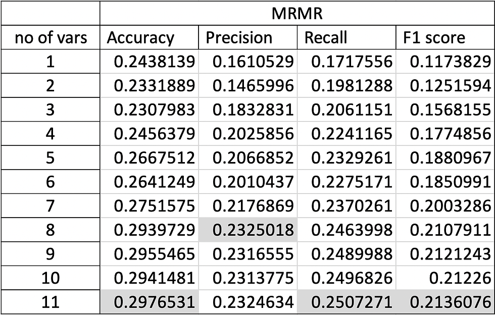
Once all the calculations were done, I put the results in an excel spreadsheet to manage them freely. For each encoding technique, I did a different table containing the result of each technique and the number of variables analyzed for example:

Table showing the results of performance metrics using MRMR technique from Ordinal Encoding
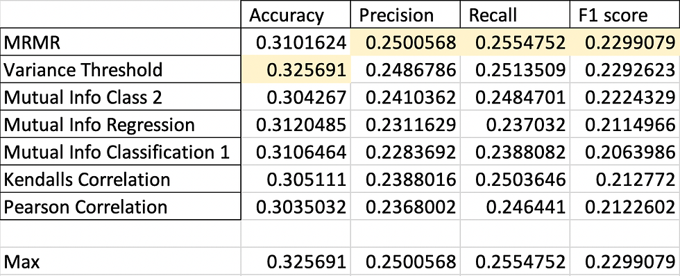
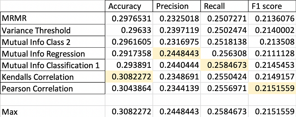
As you can see in the image above the biggest values are highlighted. Feel free to take a look at the whole document in the GitHub. Next let me present you a summary of the highest values from each technique
Manual Encoding:

One Hot Encoding:

Ordinal Encoding:

Choosing the best encoding technique and feature selection mechanism:
Let me give you the winners for each performance metric first:
Accuracy: One Hot Encoding /MRMR/3 vars
Precision: Manual Encoding/ MRMR/11 vars
Recall: Ordinal Encoding/Mutual Information Class/11 vars
F1: One Hot Encoding/Variance Threshold/18 vars
As you can see, there is no general method that outperforms the rest. This is the idea behind No Free Lunch Theorem. So let's make some analysis. Let’s say we would like to choose the best technique and the best combination of variables that will ensure that our multiclass model will have the best performance when optimizing for the smallest quantity of False Negatives, in this case, we would choose the best recall that in this case is achieved with 11 variables given by Mutual Information Classification technique and using Ordinal Encoding.
For another example, let’s say that in our model the most important parameter to optimize will be the number of False Positives, in this case, we will look for the best Precision which is given by 11 variables in the order dictated by MRMR using our Manual Encoding.
In our case, we will be using accuracy. Still, before we continue, in our next post we will try to improve the performance metrics by modifying a little more the classes inside our target variable, as 30% accuracy is extremely low.
Thanks for reading!


Comments